

Most ML engineers think about improving models during training.
But in production systems, that’s not where the real cost lives.
In modern ML workloads especially LLMs- inference is the dominant bottleneck. It drives latency, cost, scalability, and user experience. In many real-world systems, up to 80–90% of ML cost comes from inference.
Yet inference is still often treated as an afterthought.
This article is a systems-level breakdown of how to think about inference optimization—not as isolated techniques, but as a layered system problem.
A Mental Model for Inference Optimization
I like to think of inference optimization as a stack of four layers:
Model Efficiency (what you deploy)
Attention & Memory Efficiency (how the model processes tokens)
Runtime & Serving Efficiency (how requests are scheduled)
Hardware Utilization (what runs it)
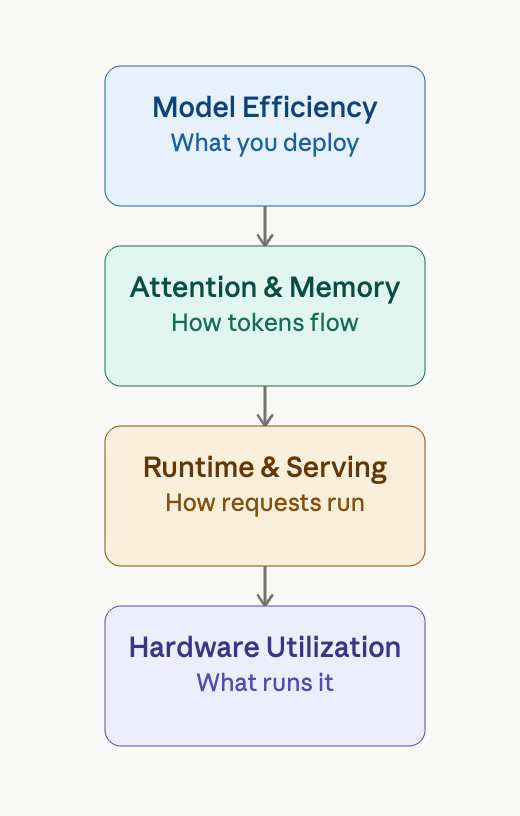
Each layer targets a different bottleneck: compute, memory, latency, or throughput.
Optimizing only one layer is not enough in production systems.
Why Inference Becomes the Bottleneck
Before optimization, it’s important to understand what we’re fighting.
1. Compute Cost
Large models require billions of operations per request.
2. Memory Bandwidth (often the real bottleneck)
For LLMs, moving data (weights + KV cache) is often more expensive than computation itself.
3. Memory Footprint
Model weights + intermediate activations + KV cache quickly exhaust GPU memory.
4. I/O and Serving Overhead
Request routing, batching, and networking add non-trivial overhead at scale.
Model-Level Optimizations: Make the Model Cheaper
This layer focuses on reducing computation and memory before inference even starts.
Quantization
Reduce numerical precision (FP32 → FP16 / INT8 / INT4).
Why it works:
Less memory usage
Faster computation
Lower bandwidth pressure
Tradeoff: Accuracy vs speed/size
Key approaches:
Post-training quantization (PTQ): fast, may lose accuracy
Quantization-aware training (QAT): better accuracy, more complex
Pruning
Remove redundant weights or connections.
Unstructured pruning: sparse weights (hard to accelerate)
Structured pruning: removes full channels/layers (hardware friendly)
Pipeline: Train → Prune → Fine-tune
Knowledge Distillation
Train a smaller model (student) to mimic a larger one (teacher).
This is one of the most practical techniques for production deployment:
Smaller model
Faster inference
Near-teacher quality
Efficient Architectures
Instead of optimizing later, design for efficiency upfront:
MobileNet / EfficientNet (CNNs)
Sparse or linear attention transformers
The Autoregressive Bottleneck
LLMs generate tokens one at a time.
This makes inference inherently sequential:
Token₁ → Token₂ → Token₃ → ...
This limits parallelism and becomes a major latency bottleneck.
Speculative Decoding
A small “draft model” proposes multiple tokens. A larger “verifier model” checks them in parallel.
Why it helps: Reduces number of expensive forward passes.
Tradeoff: Extra computation from draft model.
Medusa / Tree-based Decoding
Instead of one linear guess:
Generate multiple candidate token paths
Verify in parallel
Higher acceptance rate → better speedups.
Parallel Decoding Strategies
These methods aim to break strict token-by-token generation:
Speculative decoding (linear)
Tree-based decoding (branching)
The core idea: Trade extra compute for fewer sequential steps.
Attention & KV Cache: The Hidden Bottleneck
Attention is where many real-world systems break.
Why Attention is Expensive
Self-attention has O(L²) complexity, where L = sequence length.
This leads to:
High compute cost
Large memory usage
Poor scaling for long context
The KV Cache Problem
During decoding:
Keys and Values for all previous tokens are stored
This grows linearly with sequence length
But in practice: KV cache becomes a GPU memory bottleneck, not model weights.
Attention Optimizations
Sparse Attention
Only attend to selected tokens (local windows, global tokens, strided patterns).
Tradeoff: Global context vs efficiency.
Linear Attention
Reformulate attention to avoid O(L²), achieving O(L) complexity (may lose expressiveness).
Multi-Query / Grouped-Query Attention
Instead of separate K/V heads, share K/V across query heads.
Impact: Massive reduction in KV cache size. This directly improves:
Memory usage
Batching capacity
Throughput
PagedAttention (vLLM-style systems)
Treat KV cache like virtual memory pages.
Benefits:
Eliminates fragmentation
Improves GPU utilization
Enables large-scale batching
Hardware-Level Optimization
Inference performance is ultimately bounded by hardware.
Compute Units
GPU: best general-purpose inference engine
TPU: optimized matrix operations
NPU: edge inference
ASICs: highest efficiency, lowest flexibility
Key Insight
Modern inference systems are memory-bandwidth constrained, not compute constrained.
So hardware optimization focuses on:
Memory access speed
Data locality
Low-precision support
Runtime & Serving Optimizations
Even a perfect model can fail in a bad serving system.
Batching Strategies
Static batching: Fixed batch size → inefficient under variable load
Dynamic batching: Group requests on the fly
Continuous batching (critical for LLMs):
Processes requests as streams
Improves GPU utilization significantly
Avoids idle time
Prefill vs Decode Separation
Split inference into:
Prefill: process prompt
Decode: generate tokens step-by-step
This enables:
Separate scheduling
Better batching strategies
Optimized hardware usage
Prompt Caching
Cache repeated computations:
Embeddings
KV cache for common prefixes
Parallelism Strategies
Data Parallelism (Replica-based): Multiple copies of the model
Tensor Parallelism: Split matrix operations across GPUs
Pipeline Parallelism: Split layers across devices
Context Parallelism: Split long sequences across devices
Expert Parallelism (MoE): Activate only subset of experts per input
Compiler & Runtime Optimizations
This is where ML meets systems engineering.
Graph Optimization
Fuse ops
Remove redundancy
Reorder computation
Kernel Fusion
Combine multiple GPU operations into one kernel.
Reduces:
Kernel launch overhead
Memory movement
Memory Optimization
Efficient memory layout and reuse strategies.
Automatic Precision Conversion
Dynamic FP32 → FP16 conversion based on hardware capability.
Key Performance Metrics
Inference optimization is measured by:
Latency
Time to First Token (TTFT)
Time Per Output Token (TPOT)
Throughput
Tokens/sec or requests/sec
Resource Utilization
GPU / memory efficiency
Cost
Cost per token or per request
Closing Thought
Inference optimization is not a single technique. It is a systems problem spanning model design, memory management, scheduling, and hardware utilization.
The real shift in thinking is this:
You are no longer optimizing models. You are optimizing systems that serve models.
What’s Next
This post is the foundation. In follow-ups, we’ll go deep:
Quantization in practice: Which techniques work for which model families
Attention mechanics: Why KV cache dominates, and the tradeoffs of each optimization
Serving patterns: Building inference systems that scale
Cost modeling: How to actually measure what’s eating your budget
Let me know what you want to explore first.