
Inside the Transformer: Attention Mechanisms Deep Dive
Understanding What Happens Inside Each Layer

What We’ll Cover
In Post 1, we understood why Transformers emerged and the basic attention formula.
Now we’re going deeper:
What actually happens inside a single Transformer layer?
How do attention patterns evolve across layers?
What’s the role of feed-forward networks?
How does information flow through the entire architecture?
What are the practical engineering choices that matter?
By the end, you’ll understand:
Why Transformers have residual connections everywhere
What layer normalization actually does
How positional information propagates
The difference between encoder and decoder attention patterns
Why certain architectural choices (like pre-norm vs post-norm) matter
Let’s dive in.
1. Anatomy of a Transformer Layer
Here’s what most tutorials show you:
Input → Self-Attention → Add & Norm → Feed-Forward → Add & Norm → Output
Here’s what actually happens (and why each piece matters):
1.1 The Complete Picture
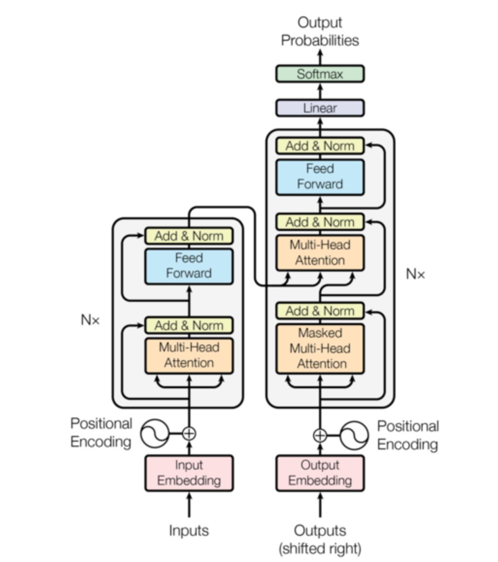
A single Transformer layer has six distinct operations:
1. Input (from previous layer or embeddings)
2. Multi-Head Self-Attention
3. Residual Connection + Dropout
4. Layer Normalization
5. Position-wise Feed-Forward Network
6. Residual Connection + Dropout + Layer Normalization
Let’s break down each component and understand why it exists.
2. Self-Attention: Beyond the Formula
In Post 1, we covered the math. Now let’s understand what it’s actually computing.
2.1 The Three Projections: Why QKV?
Every token starts as an embedding vector (say, 768 dimensions for BERT).
We project it into three different spaces:
Q = input @ W_Q  # Query: “What am I searching for?”
K = input @ W_K  # Key: “What am I advertising?”
V = input @ W_V  # Value: “What content do I provide?”
Why separate projections?
Think of it like a search engine:
Query (Q): Your search terms
Key (K): Document titles/metadata
Value (V): Document content
You match Q with K (relevance), then retrieve V (content).
The non-obvious insight: Q and K live in the same space (for dot product), but V can be in a completely different space. This separation is crucial for learning.
2.2 What Attention Scores Actually Represent
When we compute score = Q · K^T / √d_k, we’re asking:
“How much should token i care about token j?”
But here’s what’s not obvious: these scores are relative, not absolute.
After softmax, the attention distribution must sum to 1. This means:
High attention to one token → necessarily lower attention to others
Attention is a resource allocation problem
The model learns what to ignore as much as what to attend to
Example:
Sentence: “The cat sat on the mat”
Token “sat” attention: [0.05, 0.42, 0.15, 0.18, 0.08, 0.12]
The 0.42 to “cat” isn’t meaningful in isolation ,it’s meaningful because it’s much higher than 0.05 to “The” and 0.08 to “the”.
2.3 Attention Patterns Across Layers
Here’s something researchers discovered by visualizing attention in trained models:
Early layers (1-4):
Focus on local, syntactic patterns
Adjacent token attention is high
Learn basic grammar (noun-verb, determiner-noun)
Middle layers (5-8):
Learn semantic relationships
Longer-range dependencies emerge
Capture coreference, entity relationships
Late layers (9-12):
Task-specific patterns
Very focused attention (sparse patterns)
Often just propagating information
This hierarchical learning wasn’t explicitly programmed it emerged from training
2.4 The Mystery of Attention Heads
In an 8-head attention setup, here’s what researchers found heads learn:
Head 1: Might attend to the next token (positional)
Head 2: Might attend to the previous token (positional)
Head 3: Might attend to sentence boundaries
Head 4: Might focus on verbs when processing subjects
Head 5: Might track coreference (”it” → “cat”) Head 6-8: Often less interpretable, learning complex patterns
The controversial part: Not all heads are equally important. Some heads can be pruned with minimal performance loss.
Why keep 8 heads then? Redundancy and specialization.
During training, different heads explore different patterns. By the end, some become critical, others provide insurance.
3. Layer Normalization: The Unsung Hero
Layer normalization is often treated as a boring implementation detail. It’s not. It’s critical to making Transformers trainable.
3.1 What It Does
For each token, independently:
mean = x.mean(dim=-1, keepdim=True)
std = x.std(dim=-1, keepdim=True)
x_norm = (x - mean) / (std + epsilon)
output = gamma * x_norm + beta  # Learnable parameters
This normalizes across the embedding dimension (not across the batch or sequence).
3.2 Why It Matters
Problem without LayerNorm:
As you stack layers, activations can grow or shrink dramatically. By layer 12, some dimensions might be 100x larger than others. This creates:
Gradient instability
Difficulty in learning
Slow convergence
LayerNorm fixes this by keeping activations in a stable range.
3.3 Pre-Norm vs Post-Norm
This is one of those details that matters more than you’d think.
Post-Norm (Original Transformer):
x = LayerNorm(x + SelfAttention(x))
x = LayerNorm(x + FFN(x))
Pre-Norm (Modern LLMs like GPT-3):
x = x + SelfAttention(LayerNorm(x))
x = x + FFN(LayerNorm(x))
Why Pre-Norm won:
Gradient flow: Cleaner gradient path through residual connections
Stability: Easier to train very deep models (100+ layers)
No warm-up needed: Can use higher learning rates from the start
GPT-3, LLaMA, and most modern LLMs use Pre-Norm.
4. Residual Connections: Why They’re Everywhere
Every Transformer layer has two residual connections:
x = x + SelfAttention(x)
x = x + FeedForward(x)
4.1 The Gradient Superhighway
Without residual connections, the gradient for layer 1 would need to flow through:
12 self-attention blocks
12 feed-forward blocks
24 normalizations
That’s 48+ operations. Gradients would vanish.
With residual connections: The gradient can flow directly from output to input, bypassing all intermediate operations.
Think of it as:
Residual path: Gradient superhighway (direct route)
Attention/FFN path: Side roads (optional detours)
The model learns deltas (changes) rather than full transformations.
4.2 What Residual Streams Actually Learn
Here’s a mental model that helps:
Each layer adds a small update:
Layer 1: base_representation + small_update_1
Layer 2: base_representation + small_update_1 + small_update_2
...
Layer 12: base_representation + Σ(all updates)
Early layers can learn low-level features, later layers refine them, and all information is preserved through the residual stream.
This is why Transformers can be so deep , each layer makes a small, additive contribution.
5. Feed-Forward Networks: The Hidden Workhorse
After attention, every layer has a position-wise feed-forward network:
FFN(x) = max(0, x @ W1 + b1) @ W2 + b2
Two linear layers with a ReLU in between.
5.1 Why Do We Need FFN After Attention?
Attention is great at routing information between tokens. But it’s terrible at transforming that information.
Attention: “Gather relevant info from other tokens” FFN: “Process and transform that gathered info”
Think of it as:
Attention: Communication between tokens
FFN: Computation within each token
5.2 The Hidden Dimension Expansion
Here’s a key detail: the FFN has a hidden dimension that’s 4x larger than the model dimension.
For a model with d=768:
Input: 768 dimensions
Hidden layer: 3072 dimensions (4x expansion)
Output: 768 dimensions
Why expand then compress?
The expansion gives the model expressive capacity. It can compute complex, non-linear transformations in that higher-dimensional space.
Analogy: It’s like spreading out your work on a large table (3072-dim space) to do complex operations, then neatly packing it back into a small box (768-dim).
5.3 Where Parameters Live
Here’s a surprise: Most parameters are in the FFN, not attention.
For BERT-base (110M parameters):
Attention: ~25M parameters (22%)
FFN: ~75M parameters (68%)
Embeddings + other: ~10M parameters (10%)
The FFN is doing most of the heavy lifting in terms of parameter count.
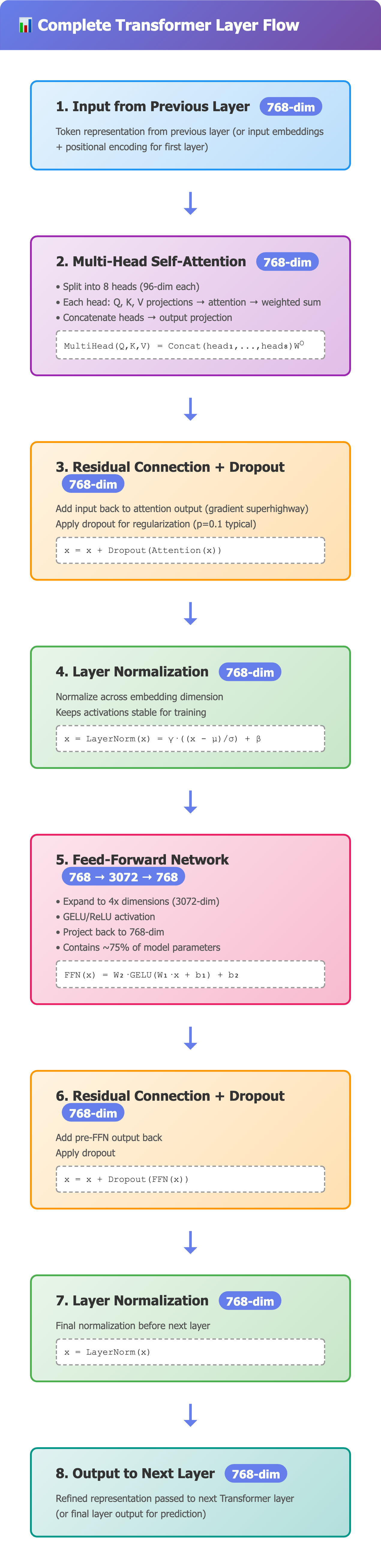
6. Complete Layer Flow: Putting It All Together
Let’s trace a single token through one Transformer layer:
1. Input: [768-dim vector]

2. Multi-Head Attention:
   - Split into 8 heads (96-dim each)
   - Each head: Q, K, V projections → attention → weighted sum
   - Concatenate 8 heads back to 768-dim
   - Output projection

3. Residual + Dropout:
   - Add input to attention output
   - Apply dropout (random zero out during training)

4. Layer Norm:
   - Normalize across 768 dimensions

5. Feed-Forward:
   - Project to 3072-dim
   - ReLU activation
   - Project back to 768-dim

6. Residual + Dropout + Layer Norm:
   - Add previous output to FFN output
   - Apply dropout
   - Normalize

7. Output: [768-dim vector] → fed into next layer
Key insight: The vector stays 768-dimensional throughout. It’s continuously being:
Mixed with other tokens (attention)
Transformed (FFN)
Refined (layer norm)
Preserved (residual connections)
7. Positional Information: How It Propagates
In Post 1, we added positional encodings at the input. But here’s the question: how does position information survive through 12 layers?
7.1 Positional Encodings Don’t Disappear
Once added at the input, positional information flows through:
Residual connections: Preserve the original positional signal
Attention: Can learn position-dependent patterns (e.g., “pay more attention to nearby tokens”)
FFN: Can condition transformations on position
The model learns to use positional information, but it’s not forced to.
7.2 Modern Alternatives: RoPE (Rotary Position Embeddings)
Models like LLaMA use RoPE instead of sinusoidal encodings.
Key difference:
Sinusoidal: Add position info to embeddings
RoPE: Rotate Q and K vectors based on position
Why RoPE is better:
Position info is baked into the attention mechanism itself
Better extrapolation to longer sequences
Relative position is more naturally represented
Formula (simplified):
Q_rotated = rotate(Q, position_m)
K_rotated = rotate(K, position_n)
attention_score = Q_rotated · K_rotated^T
The dot product automatically captures relative position (m - n).
8. Encoder vs Decoder: Attention Pattern Differences
8.1 Encoder (BERT-style): Bidirectional Attention
Every token can attend to every other token, including future tokens.
“The cat sat on the mat”

“cat” can attend to: [The, cat, sat, on, the, mat]
Use case: Understanding tasks (classification, NER, Q&A) You need full context to understand meaning.
8.2 Decoder (GPT-style): Causal Attention
Token i can only attend to tokens 1...i (no peeking at future).
This is enforced via an attention mask:
Attention mask (lower triangular):
1 0 0 0 0 0
1 1 0 0 0 0
1 1 1 0 0 0
1 1 1 1 0 0
1 1 1 1 1 0
1 1 1 1 1 1
Before softmax, we set masked positions to -∞, so they get zero attention.
Why causal? For autoregressive generation (predicting next token), the model shouldn’t cheat by looking ahead.
8.3 Encoder-Decoder (T5-style): Cross-Attention
Decoder attends to encoder outputs:
Encoder: Processes input bidirectionally
Decoder:
  - Self-attention (causal) on output tokens
  - Cross-attention to encoder outputs
  - Generates output autoregressively
Cross-attention mechanism:
Q: From decoder
K, V: From encoder outputs
This allows the decoder to “look at” the input while generating output.
9. What Makes Attention “Learn”?
9.1 Attention is Learned, Not Programmed
The matrices W^Q, W^K, W^V are learned through backpropagation.
Initially (random initialization):
Attention is nearly uniform
All tokens attend equally to all others
Model is useless
During training:
Gradients flow through attention scores
Model learns: “When I see X, attend strongly to Y”
Useful patterns emerge
The model discovers that:
Verbs should attend to subjects
Pronouns should attend to their referents
Adjectives should attend to nouns
etc.
None of this is hardcoded.
9.2 The Softmax Bottleneck
Here’s a limitation not often discussed:
Softmax forces attention to be a probability distribution (sums to 1).
This creates a bottleneck:
If you need to attend strongly to 5 tokens, each gets ~0.2 attention
If you need to attend to 1 token, it gets ~1.0 attention
For very long sequences, this becomes problematic. You might need information from 10 different tokens, but softmax forces you to distribute attention thinly.
Solutions in research:
Sparse attention (attend to subsets)
Multi-query attention (share K, V across heads)
Attention alternatives (Mamba, RWKV)
10. Engineering Choices That Matter
10.1 Dropout Placement
Dropout is applied in three places:
After attention output projection
After FFN output projection
Sometimes on attention weights themselves
Why? Regularization. Prevents overfitting by randomly dropping connections during training.
Typical values: 0.1 (drop 10% of activations)
10.2 Activation Functions
Original Transformer: ReLU in FFN Modern LLMs: GELU (Gaussian Error Linear Unit) or SwiGLU
Why GELU?
Smoother gradients
Better empirical performance
Used in BERT, GPT-3, etc.
Formula:
GELU(x) = x * Φ(x) where Φ is Gaussian CDF
Approximately: 0.5 * x * (1 + tanh(√(2/π) * (x + 0.044715 * x³)))
10.3 Initialization
Getting initialization right is crucial:
Xavier/Glorot initialization:
W ~ N(0, 2/(d_in + d_out))
Why it matters:
Too small → vanishing activations
Too large → exploding activations
Modern Transformers often use scaled initialization where deeper layers get smaller initial weights.
10.4 Learning Rate Schedules
Warmup + Decay:
1. Linear warmup: 0 → max_lr (first 4000-10000 steps)
2. Inverse square root decay: lr ∝ 1/√step
Why warmup? Early in training, large gradients can destabilize the model. Warmup lets the model “settle” before full-speed training.
11. Visualizing Attention: What Works, What Doesn’t
11.1 Attention Heatmaps
Common visualization: plot attention weights as a matrix.
What it shows: Which tokens attend to which What it doesn’t show: What information is actually extracted
Limitation: High attention ≠ high importance for the final prediction
11.2 Better Interpretability Methods
1. Attention Rollout Combine attention across layers to see end-to-end paths
2. Gradient-based Attribution Which tokens, when changed, most affect the output?
3. Probing Classifiers Train simple classifiers on layer outputs to see what information is encoded
4. Causal Interventions Ablate specific attention heads and measure impact
12. Common Misconceptions Revisited
Misconception #1: “Each layer builds higher-level features”
Reality: Not always hierarchical. Later layers sometimes undo earlier work or route around it via residual connections.
Misconception #2: “More heads = better”
Reality: Diminishing returns. 16 heads isn’t 2x better than 8. Some research shows 4-8 heads is a sweet spot.
Misconception #3: “Attention does all the work”
Reality: FFN has 3x more parameters and is equally critical. Attention routes information; FFN processes it.
Misconception #4: “Layer norm is just a regularization trick”
Reality: It’s fundamental to training stability. Without it, deep Transformers are nearly untrainable.
13. Interview Deep-Dive: Architecture Questions
Q1: Walk me through one forward pass of a Transformer layer.
Answer:
Input (d-dim) → Multi-head attention
Add input back (residual) → Layer norm
FFN: d → 4d → d with ReLU
Add previous output (residual) → Layer norm
Output passed to next layer
Key: Residual connections provide gradient paths; layer norm stabilizes training.
Q2: Why do we need separate Q, K, V projections?
Answer: Attention is computing a weighted sum. Q and K determine weights (via dot product), V provides content. Separating them gives the model flexibility: relevance (Q·K) and content (V) can be learned independently. If we used the same projection, attention would be symmetric and less expressive.
Q3: What’s the purpose of the FFN after attention?
Answer: Attention is linear in content (weighted sum). FFN adds non-linearity and transformation capacity. Attention routes information between tokens; FFN processes information within each token. Without FFN, the model would be limited to linear combinations.
Q4: Pre-norm vs post-norm, which is better and why?
Answer: Pre-norm is better for deep models:
Cleaner gradient flow through residuals
More stable training (no warmup needed)
Used in GPT-3, LLaMA, modern LLMs
Post-norm was original design but struggles with very deep models (>24 layers).
Q5: How does positional information propagate through layers?
Answer: Added at input, then:
Residual connections preserve original positional encodings
Attention can learn position-dependent patterns
Model learns to use or ignore position as needed per layer
Modern approach (RoPE): Rotate Q/K based on position, baking positional info into attention mechanism directly.
Q6: What happens during causal masking in decoder attention?
Answer: Before softmax, set future positions to -∞:
scores = QK^T / √d_k
scores[i, j] = -∞ where j > i  # Mask future
attention = softmax(scores)  # Future positions → 0
This prevents token i from attending to tokens after position i, enforcing autoregressive property.
Q7: Why is √d_k important in scaled dot-product attention?
Answer: Dot product magnitude grows with dimension. For d_k = 512, unscaled dot products can be large (±50), pushing softmax into saturation (extreme outputs like 0.0001, 0.9998). This kills gradients.
Dividing by √d_k normalizes variance to ~1, keeping softmax in its “soft” regime where gradients are healthy. Critical for trainability.
Q8: How much compute does self-attention use vs FFN?
Answer: Per layer for sequence length n, model dim d:
Self-attention: O(n² · d) for attention matrix + O(n · d²) for projections
FFN: O(n · d²) typically (d → 4d → d)
For short sequences (n < d), FFN dominates compute. For long sequences (n > d), attention dominates.
In practice: FFN has 3x more parameters but attention has quadratic complexity in n.
Q9: Can you remove attention heads without hurting performance?
Answer: Yes, to some extent. Research shows:
Some heads are redundant (10-20% can be pruned)
But most heads contribute something unique
Pruning requires careful analysis (can’t just randomly remove)
Some tasks more sensitive than others
Suggests multi-head attention has useful redundancy but isn’t wasteful.
Q10: What’s the memory bottleneck during inference?
Answer: KV cache. For autoregressive generation:
Store K, V for all previous tokens
At each step, attend to cached K, V
Memory: O(n · layers · d) per sequence For 2K context, 32 layers, d=4096: ~1GB per request
This is why context length is expensive—it’s primarily a memory problem, not compute.
14. Practical Takeaways
For Building Systems:
Pre-norm architecture for new models (better training stability)
GELU/SwiGLU activations over ReLU (better performance)
RoPE positional encoding for better extrapolation (used in LLaMA)
FlashAttention for memory-efficient training (3x faster, 10x less memory)
Gradient checkpointing to trade compute for memory
For Understanding Models:
Attention patterns evolve across layers (syntactic → semantic → task-specific)
FFN does most computation (3x more parameters than attention)
Residual connections are critical for gradient flow
Not all attention heads are equal (some can be pruned)
Position information propagates via residuals and attention
For Debugging:
Check attention entropy (low = too focused, high = too uniform)
Visualize attention rollout for multi-layer paths
Monitor gradient norms (residuals help, but explosions still happen)
Probe intermediate layers to see what’s learned where
Ablate heads/layers to find critical components
✨ The Bigger Picture
Understanding Transformer internals isn’t just academic ,it’s practical:
For research:
Know what to modify (attention alternatives, FFN variants)
Understand scaling properties
Debug training issues
For engineering:
Optimize inference (KV cache, attention kernels)
Choose architectures (encoder vs decoder)
Tune hyperparameters meaningfully
For product:
Understand capabilities and limitations
Make informed model selection
Predict behavior on edge cases
Every layer refines the representation a bit more. Every attention head captures a different pattern. Every residual connection preserves information flow.
The beauty is in how simple components compose into powerful systems.
📚 References & Further Reading
🔹 Foundational & Core Attention Papers
Bahdanau et al. (2014) – Neural Machine Translation by Jointly Learning to Align and Translate
https://arxiv.org/abs/1409.0473Luong et al. (2015) – Effective Approaches to Attention-based Neural Machine Translation
https://arxiv.org/abs/1508.04025Vaswani et al. (2017) – Attention Is All You Need (for multi-head attention formalization)
https://arxiv.org/abs/1706.03762
🔹 Technical Deep Dives & Visual Guides
Jay Alammar – The Illustrated Attention
https://jalammar.github.io/visualizing-neural-machine-translation-mechanisms-and-attention/The Illustrated Transformer (Attention section)
https://jalammar.github.io/illustrated-transformer/Lilian Weng – Attention? Attention!
https://lilianweng.github.io/posts/2018-06-24-attention/Harvard NLP – Annotated Transformer (Attention code walkthrough)
http://nlp.seas.harvard.edu/annotated-transformer/Peter Bloem – Transformers from Scratch (detailed math on attention)
https://peterbloem.nl/blog/transformers
🔹 Research & Variants of Attention
Sparse Transformers (OpenAI, 2019)
https://arxiv.org/abs/1904.10509Performer: Linear Attention (Choromanski et al., 2020)
https://arxiv.org/abs/2009.14794Longformer (Beltagy et al., 2020) – Local + Global attention pattern
https://arxiv.org/abs/2004.05150Linformer (Wang et al., 2020) – Low-rank self-attention
https://arxiv.org/abs/2006.04768
🔹 Videos & Talks
Yannic Kilcher – Attention Mechanisms Explained
Andrew Ng – Self-Attention Explanation (DeepLearning.AI)
MIT 6.S191 – Lecture on Attention Mechanisms
Karpathy – “Let’s Build Attention From Scratch” (implicit in GPT lecture)
What’s Next?
This post covered what happens inside a Transformer.
Next in the series:
Post 3: Scaling Laws & Training LLMs
Post 4: Alignment & Production
If this deep-dive was valuable, share it with someone learning ML. This series documents everything I wish I understood when building with Transformers.