

Welcome back to the Deep Learning Interview Prep Series! 🚀
After mastering CNNs for images, it’s time to tackle sequential data.
Enter Recurrent Neural Networks (RNNs) the models that remember the past to understand the present. From text and speech to time-series forecasting, RNNs process sequences step by step, capturing context and patterns along the way. Let’s dive in!
1. Conceptual Understanding
Most standard neural architectures, like feedforward networks or CNNs, assume independence between inputs. That is, each input is processed in isolation. However, sequential data violates this assumption the current input often depends on prior inputs.
Examples of sequential dependencies:
Text/NLP: The meaning of a word depends on context from previous words.
E.g., in “The bank will not approve your loan,” the meaning of bank depends on context.
Time Series: Stock prices, weather, and sales data depend on previous values.
Speech/Audio: Phonemes and words are recognized based on preceding sounds.
Control Systems: Robotics and reinforcement learning require past states to decide the next action.
1.1 RNN Intuition
RNNs introduce a hidden state vector (h_t) that acts as a memory. At each time step, the network combines the current input (x_t) with the previous hidden state (h_{t-1}) to compute the new hidden state:
Where:
(x_t) - input at time step (t)
(h_t) - hidden state at time step (t)
(f) - activation function ((\tanh) or ReLU)
(W_{xh}, Whh, W_{hy}) - learnable weights

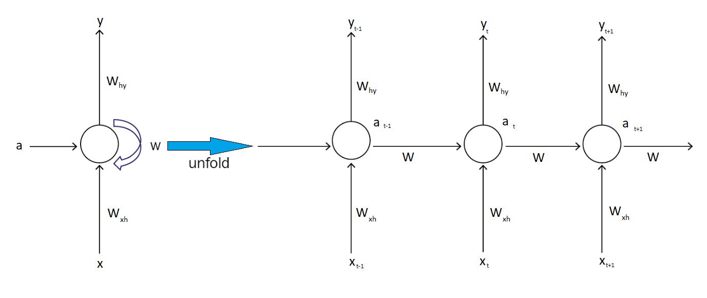
The recurrence allows information to flow across time steps, creating a chain-like dependency that can, in principle, capture long-term patterns.
1.2 Vanishing and Exploding Gradients
RNNs are trained using Backpropagation Through Time (BPTT). Gradients for weight updates are propagated across multiple time steps:
Vanishing Gradient: When the magnitude of the derivative is <1, repeated multiplications across time steps cause the gradient to shrink exponentially. As a result, the network struggles to learn long-term dependencies, because the influence of earlier inputs essentially disappears.
Exploding Gradient: When the magnitude of derivative >1, repeated multiplications cause the gradient to grow exponentially. This can lead to unstable training, with huge weight updates and numerical overflow.
Practical Solutions:
Gradient clipping: Limit gradients to a maximum norm to avoid explosion.
Use LSTM/GRU cells: Gated architectures mitigate vanishing gradients.
Proper initialization: Orthogonal or Xavier initialization helps stabilize gradients.
2. Applied Perspective
RNNs are suitable for sequential tasks but come with trade-offs.
2.1 Applications
Natural Language Processing (NLP):
Language modeling, text generation, sentiment analysis, machine translation.
Example: Predict the next word given previous words.
Speech Recognition: Convert audio sequences to text.
Example: “hello world” recognized from audio frames.
Time Series Forecasting: Sales, temperature, stock prices.
Control Systems & Robotics: Sequential decision-making based on past states.
2.2 Limitations
Poor performance on very long sequences.
Sequential dependency slows training; cannot parallelize like CNNs or Transformers.
Mostly replaced by Transformers in large-scale NLP.
2.3 When RNNs Still Make Sense
Small-to-medium datasets.
Moderate sequence length (<100 time steps).
Deployments in edge devices or low-compute environments.
3. System Design Perspective
When designing a system for sequential data, choosing the right architecture is all about trade-offs:
RNNs are simple and lightweight great for short sequences, but struggle when context from far back matters.
LSTMs solve that by using gated memory to capture long-range dependencies, though they come with more parameters and slower training.
GRUs strike a balance - faster and lighter than LSTMs, handling medium-length sequences efficiently, with slightly less expressiveness.
Transformers take it to the next level, using global attention to learn from long sequences and parallelize computation- but they need more data and compute power.
In short: RNNs for small, quick tasks, LSTMs/GRUs for medium sequences, and Transformers for large-scale sequence learning.
3.1 Example: RNN for Sentiment Classification
Pipeline:
Tokenize text → convert to embeddings.
Feed sequence into RNN → hidden states (h_1, h_2, ..., h_T).
Use last hidden state (h_T) as feature for classification.
Dense layer + softmax → probability for positive/negative sentiment.
Notes:
Can use bidirectional RNNs to capture context from both past and future.
Truncated BPTT: for long sequences, backpropagation is limited to last N steps to save memory and compute.
3.2 Practical Tips for Training RNNs
Use gradient clipping to avoid exploding gradients.
Consider layer normalization for stability.
Use pre-trained embeddings (GloVe, Word2Vec) for NLP.
Experiment with bidirectional RNNs for context from both past and future.
Use truncated BPTT for long sequences.
4. Detailed Math: Backpropagation Through Time (BPTT)
Consider a loss (L) over the sequence:
Gradient w.r.t hidden state (h_t):
This recursive structure highlights why:
Gradients vanish: product goes to zero.
Gradients explode: product grows exponentially.
Truncated BPTT: Only backpropagate through last (k) steps, balancing memory and gradient flow.
5. RNN Variants
5.1 LSTM
Components:
Forget gate: decides what to discard from memory.
Input gate: decides what new information to store.
Output gate: decides what part of memory to output.

ft -forget gate
it - input gate
ot - output gate
C~t - candidate cell state
Ct - current cell state
ht - hidden state / output
5.2 GRU
Combines forget & input gates into update gate.
Uses reset gate to control new information.

zt - update gate
rt - reset gate
h~t - candidate hidden state
ht - final hidden state at time t
6. Interview Questions
What is the difference between RNN, LSTM, and GRU?
Why do RNNs suffer from vanishing gradients?
Explain Backpropagation Through Time (BPTT).
When would you use an RNN over a Transformer?
How does parameter sharing in RNNs compare to CNNs?
7. Solutions
Q1. What is the difference between RNN, LSTM, and GRU?
Answer:
RNN: Simple recurrence, maintains short-term memory, struggles with long-term dependencies.
LSTM: Uses input, forget, and output gates to regulate memory, effectively handles long-term dependencies, mitigates vanishing gradients.
GRU: Combines gates into update and reset gates, fewer parameters, faster than LSTM, handles medium-length dependencies efficiently.
Q2. Why do RNNs suffer from vanishing gradients?
Answer:
During backpropagation, the gradient at each time step is a product of many small derivatives. If these derivatives are less than 1, the gradient shrinks exponentially across time steps, making it hard to learn long-term dependencies.
Q3. Explain Backpropagation Through Time (BPTT).
Answer:
Unroll the RNN over all time steps.
Perform a forward pass to compute outputs and loss.
Use the chain rule to backpropagate gradients through time.
Truncated BPTT can be used to limit unrolling for long sequences to save memory and computation.
Q4. When would you use an RNN over a Transformer?
Answer:
When the dataset is small.
In low-compute environments or edge devices.
For short to medium-length sequences where Transformers are overkill.
Q5. How does parameter sharing in RNNs compare to CNNs?
Answer:
RNNs: Parameters are shared across time steps, allowing the network to generalize across sequences.
CNNs: Parameters are shared across spatial locations, enabling feature detection across the input space.
Conclusion
RNNs were the first major deep learning breakthrough for sequential data, enabling models to process information across time steps. They laid the groundwork for LSTMs, GRUs, and attention-based architectures.
While vanilla RNNs struggle with long-term dependencies due to vanishing gradients, they remain valuable for medium-length sequences, small datasets, and resource-constrained environments. Mastering RNNs builds a strong foundation for understanding modern sequence models in NLP, time series, and speech applications.
Next in the Series
Next, we’ll explore Advanced Sequence Models, diving into:
Bidirectional RNNs – capturing context from both past and future.
Seq2Seq architectures – encoder-decoder frameworks for translation and summarization.
Attention mechanism – the stepping stone to Transformers.
These concepts set the stage for Transformers and large-scale sequence modeling, connecting classical RNNs to state-of-the-art architectures.